Comparing the performance of different regressors with the goal of predicting housing prices from the number of rooms. Dataset Used: Boston Housing Data

Introducing the Data

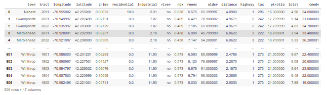
The Boston Housing dataset is a collection from the U.S. Census Service concerning Boston, MA’s housing. The dataset has 506 total data points and 17 attributes. The Dataset’s attributes are listed as follows:

1. crime - per capita crime rate by town
2. residential - proportion of residential land zoned for lots over 25,000 sq.ft.
3. industrial - proportion of non-retail business acres per town.
4. river - Charles River dummy variable (1 if tract bounds river; 0 otherwise)
5. nox - nitric oxides concentration (parts per 10 million)
6. rooms - average number of rooms per dwelling
7. older - proportion of owner-occupied units built prior to 1940
8. distance - weighted distances to five Boston employment centres
9. highway - index of accessibility to radial highways
10. tax - full-value property-tax rate per $10,000
11. ptratio - pupil-teacher ratio by town
12. town
13. lstat - % lower status of the population
14. cmedv - Median value of owner-occupied homes in $1000’s
15. tract - year
16. longitude
17. latitude

Establishing a Data Frame

In order to access the data in Colab, we must first upload the dataset to google drive and then mount the drive on Colab:

from google.colab import drive
drive.mount('/content/drive')

Once the data is accessible, we must import the libraries needed to create a data frame:

import numpy as np
import pandas as pd
import matplotlib as mpl
import matplotlib.pyplot as plt

Then, we create the data frame. If we do not need to clean it up or make any adjustments, we can move on to the next step:

df = pd.read_csv('drive/MyDrive/BostonHousingPrices.csv')

This particular project will explore the relationship between rooms and housing prices.

Visualizing the Data

In order to get a better perspective on what type of regression may be best for our model, let’s plot out the two attributes:

%matplotlib inline
%config InlineBackend.figure_format = 'retina' #Formats the visual representation
fig, ax = plt.subplots(figsize=(10,8)) #handles the size of plot

ax.set_xlim(3, 9) #boundaries of x
ax.set_ylim(0, 51) #boundaries of y

ax.scatter(x=df['rooms'], y=df['cmedv'],s=25) #plots the points

ax.set_xlabel('Number of Rooms',fontsize=16,color='darkgreen') #labels for x
ax.set_ylabel('House Price (Thousands of Dollars)',fontsize=16,color='darkgreen') #labels for y
ax.set_title('Boston Housing Prices',fontsize=18,color='purple') #plot label

ax.grid(b=True,which='major', color ='grey', linestyle='-', alpha=0.8) #sets grid
ax.grid(b=True,which='minor', color ='grey', linestyle='--', alpha=0.2)
ax.minorticks_on()
plt.show()

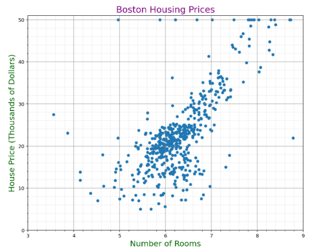
The plot seems to show at first glance a positive increasing linear trend. However, we also note that there are large clusters and a lot of noise, possibly making this a difficult dataset to model.

Prediction Modeling

Prediction Modeling in Machine Learning requires one to split the data into a training set and testing set. The parameters chosen are largely dependent on the problem at hand and the data set itself. There are many types of prediction models we can apply to data, some being more accurate than others. One way to measure a model’s accuracy is through the MAE or Mean Absolute Error. This error metric is essentially the sum of all absolute errors in the model’s predictions. Absolute Errors take the absolute value of the difference between an actual value and the predicted value. On a plot, we can measure the MAE as the average vertical distance between each point and the predicted line. The smaller the error, the better the predictive model.

Linear Regression Predictive Model

Our problem type deems it necessary to derive a continuous numerical value as our predicted value. The nature of our problem thus makes a linear regression algorithm a great candidate for our predictive model. Linear Regressions establish a linear relationship between and independent variable x and dependent variable y. Linear Regressions find the line of best fit in the data and use this to predict future values. In order to find the line of best fit, optimization algorithms such as gradient descent are used. Outliers in the data may cause overfitting of the linear regression, thus lowering the overal testing accuracy.

Linear Regression models are statistical models, but how do they differ from statistical analysis? While in statistics we calculate the unknowns using statistical formulas, linear regression in machine learning only uses optimization algorithms. For example, assuming we have several dimensions of variables, statistical analysis will tell us to find our beta values (correlation coefficients) and any constants or intercepts. Machine learning will find these values by simply minimizing error.

Linear Regression not only helps one predict variables but also quantify the impact independent variables have on the dependent variable as well as identifying the most important variables.

Modeling Linear Regressions in Python

In order to begin with our model, we must first indicate our independent and dependent variables and seperate the data into training and testing sets.

from sklearn.model_selection import train_test_split
X = np.array(df['rooms']).reshape(-1,1)
y = np.array(df['cmedv']).reshape(-1,1)

We will choose a test size of 0.3 and random state 2021 in order to have consistency across all models.

X_train, X_test, y_train, y_test = train_test_split(X, y, test_size=0.3, random_state=2021)

y_train = y_train.reshape(len(y_train),)
y_test = y_test.reshape(len(y_test),)

Lastly, we will apply the linear regression model from the sklearn library.

from sklearn.linear_model import LinearRegression
lm = LinearRegression()
lm.fit(X_train, y_train)

Analyzing our Model

As mentioned earlier, we can use mean absolute error in order to determine the accuracy of our model. We can import the mean absolute error package from sklearn to determine the deviation from the actual value and predicted value.

from sklearn.metrics import mean_absolute_error 
print("Intercept: {:,.3f}".format(lm.intercept_))
print("Coefficient: {:,.3f}".format(lm.coef_[0]))
    
mae = mean_absolute_error(y_test, lm.predict(X_test))
print("MAE = ${:,.2f}".format(1000*mae))

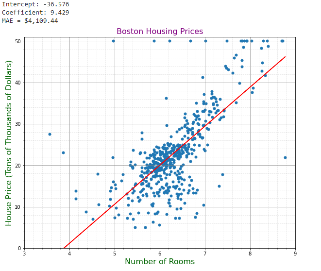
We can also plot our linear regression:

fig, ax = plt.subplots(figsize=(10,8))
ax.set_xlim(3, 9)
ax.set_ylim(0, 51)
ax.scatter(x=df['rooms'], y=df['cmedv'],s=25)
ax.plot(X_test, lm.predict(X_test), color='red') #linear regression
ax.set_xlabel('Number of Rooms',fontsize=16,color='Darkgreen')
ax.set_ylabel('House Price (Tens of Thousands of Dollars)',fontsize=16,color='Darkgreen')
ax.set_title('Boston Housing Prices',fontsize=16,color='purple')
ax.grid(b=True,which='major', color ='grey', linestyle='-', alpha=0.8)
ax.grid(b=True,which='minor', color ='grey', linestyle='--', alpha=0.2)
ax.minorticks_on()

Linear Regression

The Model has an MAE of $4,109.44. Our linear regression model has a rather high MAE, thus making this a weak learner. Because of the clustering of data points in an unlinear fashion, our model may have lost accuracy trying to fit such points.

Kernel Weighted Local Regression

LOWESS or locally weighted linear regressions are non-parametric regressions in which the simplicity of a linear regression is combined with the flexibility of non linear regression. LOWESS regressions are used when there are non-linear relationships between variables. In essence, linear functions using weighted least squares are fitted only on local sets of data, thus building up to a function that describes the overall variation. For each value of x, the value of f(x) is estimated using its neighboring known values.

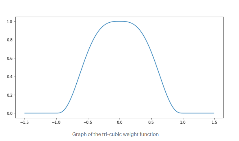
Let us say we choose a specific data set point X1 for which we want to predict its Y1 value. We can determine its neighbors by choosing a specific distance which will result in some ordered set A. This set will be converted into another weighted set using a weight/kernel function. The specific weights will depend on what kernel function is chosen. Example: Below we have chosen a tri-cubic function as our weight function.

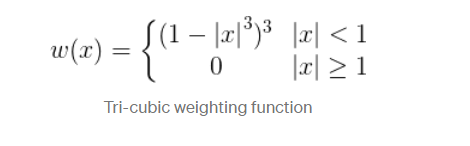
The heights of the kernel function determine the weights at specific points. The neighbors closer to the target point X1 will have higher weights than points further away. In other words, by locally weighing points, we can assign higher importance to training data that is closest to the target point.

For every target point X1, LOWESS will apply a linear regression that will calculate the corresponding Y1 value. Although this algorithm may work well for regression applications with complex deterministic structures, LOWESS has several disadvantages. Because a model is computed for each point, it is very computationally intensive as well as having a large parameter size. It is still quite volatile to outliers in the data set as well as it cannot be translated into a mathematical formula.

Modeling Locally Weighted Linear Regressions in Python

LOESS regressions only require kernel functions and smoothening/bandwidth parameters. Thus, we must define several kernel functions.

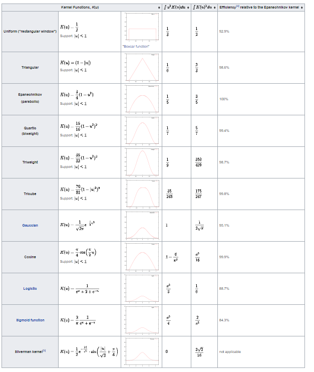
Epanechnikov Kernel

We begin by importing necessary libraries:

import numpy as np
import pandas as pd
from math import ceil
from scipy import linalg
from scipy.interpolate import interp1d
import matplotlib.pyplot as plt

Next, we must define the Epanechnikov function Pythonically:

def Epanechnikov(x):
  return np.where(np.abs(x)>1,0,3/4*(1-np.abs(x)**2)) 

We must also define the LOWESS kernel function which will take in x & y parameters as well as kernel function and bandwidth parameters:

def lowess_kern(x, y, kern, tau):
    n = len(x)
    yest = np.zeros(n)

    #Initializing all weights from the kernel function by using only the train data    
    w = np.array([kern((x - x[i])/(2*tau)) for i in range(n)])     
    
    #Looping through all x-points
    for i in range(n):
        weights = w[:, i]
        b = np.array([np.sum(weights * y), np.sum(weights * y * x)])
        A = np.array([[np.sum(weights), np.sum(weights * x)],
                    [np.sum(weights * x), np.sum(weights * x * x)]])
        theta, res, rnk, s = linalg.lstsq(A, b)
        yest[i] = theta[0] + theta[1] * x[i] 

    return yest

LOWESS Regressions require one to sort the data to create a matrix:

dat = np.concatenate([X_train,y_train.reshape(-1,1)], axis=1) #matrix of two columns

# this is sorting the rows based on the first column
dat = dat[np.argsort(dat[:, 0])]

dat_test = np.concatenate([X_test,y_test.reshape(-1,1)], axis=1)
dat_test = dat_test[np.argsort(dat_test[:, 0])]

Lastly, we must call the Lowess Function with its corresponding kernel (Epanechnikov) and a bandwidth of 0.05 and predict on the test set.

Yhat_lowess = lowess_kern(dat[:,0],dat[:,1],Epanechnikov,0.05) #CHOOSE KERNEL
datl = np.concatenate([dat[:,0].reshape(-1,1),Yhat_lowess.reshape(-1,1)], axis=1)

f = interp1d(datl[:,0], datl[:,1],fill_value='extrapolate')
yhat = f(dat_test[:,0])

We can assess the accuracy in terms of the MAE and compare it to our Linear Regression:

from sklearn.metrics import mean_absolute_error 
    
mae_lowess = mean_absolute_error(dat_test[:,1], yhat)
print("MAE LOWESS = ${:,.2f}".format(1000*mae_lowess))

# Plot outputs
fig, ax = plt.subplots(figsize=(10,8))
ax.set_xlim(3, 9)
ax.set_ylim(0, 51)
ax.scatter(x=df['rooms'], y=df['cmedv'],s=25)
ax.plot(dat_test[:,0], yhat, color='orange',lw=3) #LOWESS
ax.set_xlabel('Number of Rooms',fontsize=16,color='Darkgreen')
ax.set_ylabel('House Price (Tens of Thousands of Dollars)',fontsize=16,color='Darkgreen')
ax.set_title('Boston Housing Prices',fontsize=16,color='purple')
ax.grid(b=True,which='major', color ='grey', linestyle='-', alpha=0.8)
ax.grid(b=True,which='minor', color ='grey', linestyle='--', alpha=0.2)
ax.minorticks_on()

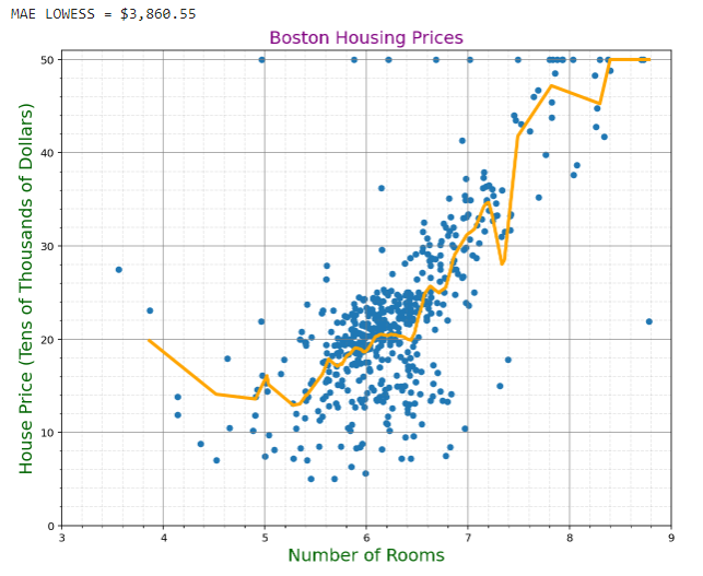
We can see that the LOWESS MAE is smaller than that of the linear regression at $3,860.55. This is still relatively high, but much better than our previous approach.

Quartic Kernel

We can do the same steps above with a different kernel and analyze its accuracy:

import numpy as np
import pandas as pd
from math import ceil
from scipy import linalg
from scipy.interpolate import interp1d
import matplotlib.pyplot as plt

def Quartic(x):
  return np.where(np.abs(x)>1,0,15/16*(1-np.abs(x)**2)**2) 
  
def lowess_kern(x, y, kern, tau):
    n = len(x)
    yest = np.zeros(n)

    #Initializing all weights from the kernel function by using only the train data    
    w = np.array([kern((x - x[i])/(2*tau)) for i in range(n)])     
    
    #Looping through all x-points
    for i in range(n):
        weights = w[:, i]
        b = np.array([np.sum(weights * y), np.sum(weights * y * x)])
        A = np.array([[np.sum(weights), np.sum(weights * x)],
                    [np.sum(weights * x), np.sum(weights * x * x)]])
        theta, res, rnk, s = linalg.lstsq(A, b)
        yest[i] = theta[0] + theta[1] * x[i] 

    return yest
    
dat = np.concatenate([X_train,y_train.reshape(-1,1)], axis=1)
#matrix of two columns

# this is sorting the rows based on the first column
dat = dat[np.argsort(dat[:, 0])]

dat_test = np.concatenate([X_test,y_test.reshape(-1,1)], axis=1)
dat_test = dat_test[np.argsort(dat_test[:, 0])]  
    
Yhat_lowess = lowess_kern(dat[:,0],dat[:,1],Quartic,0.05) #CHOOSE KERNEL
datl = np.concatenate([dat[:,0].reshape(-1,1),Yhat_lowess.reshape(-1,1)], axis=1)
f = interp1d(datl[:,0], datl[:,1],fill_value='extrapolate')
yhat = f(dat_test[:,0])


from sklearn.metrics import mean_absolute_error 

mae_lowess = mean_absolute_error(dat_test[:,1], yhat)
print("MAE LOWESS = ${:,.2f}".format(1000*mae_lowess))

# Plot outputs
fig, ax = plt.subplots(figsize=(10,8))
ax.set_xlim(3, 9)
ax.set_ylim(0, 51)
ax.scatter(x=df['rooms'], y=df['cmedv'],s=25)
ax.plot(dat_test[:,0], yhat, color='orange',lw=3) #LOWESS
ax.set_xlabel('Number of Rooms',fontsize=16,color='Darkgreen')
ax.set_ylabel('House Price (Tens of Thousands of Dollars)',fontsize=16,color='Darkgreen')
ax.set_title('Boston Housing Prices',fontsize=16,color='purple')
ax.grid(b=True,which='major', color ='grey', linestyle='-', alpha=0.8)
ax.grid(b=True,which='minor', color ='grey', linestyle='--', alpha=0.2)
ax.minorticks_on()

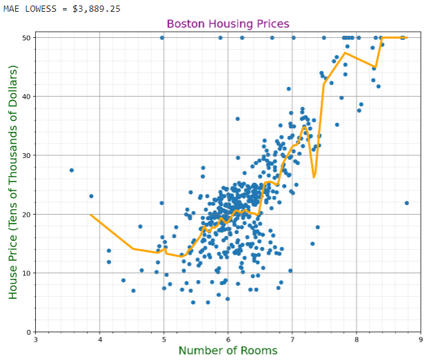
The Quartic Kernel LOWESS offers a MAE of $3,889.25, which is a bit higher than that of the Epanechnikov Kernel, thus making it not as accurate.

Tri-Cubic Kernel

We shall now try the Tri-cubic kernel in LOWESS.

import numpy as np
import pandas as pd
from math import ceil
from scipy import linalg
from scipy.interpolate import interp1d
import matplotlib.pyplot as plt

# Tricubic Kernel
def tricubic(x):
  return np.where(np.abs(x)>1,0,70/81*(1-np.abs(x)**3)**3)
  
def lowess_kern(x, y, kern, tau):
    n = len(x)
    yest = np.zeros(n)

    #Initializing all weights from the kernel function by using only the train data    
    w = np.array([kern((x - x[i])/(2*tau)) for i in range(n)])     
    
    #Looping through all x-points
    for i in range(n):
        weights = w[:, i]
        b = np.array([np.sum(weights * y), np.sum(weights * y * x)])
        A = np.array([[np.sum(weights), np.sum(weights * x)],
                    [np.sum(weights * x), np.sum(weights * x * x)]])
        theta, res, rnk, s = linalg.lstsq(A, b)
        yest[i] = theta[0] + theta[1] * x[i] 

    return yest

dat = np.concatenate([X_train,y_train.reshape(-1,1)], axis=1)
#matrix of two columns

# this is sorting the rows based on the first column
dat = dat[np.argsort(dat[:, 0])]

dat_test = np.concatenate([X_test,y_test.reshape(-1,1)], axis=1)
dat_test = dat_test[np.argsort(dat_test[:, 0])] 

Yhat_lowess = lowess_kern(dat[:,0],dat[:,1],tricubic,0.05) #CHOOSE KERNEL
datl = np.concatenate([dat[:,0].reshape(-1,1),Yhat_lowess.reshape(-1,1)], axis=1)
f = interp1d(datl[:,0], datl[:,1],fill_value='extrapolate')
yhat = f(dat_test[:,0])

from sklearn.metrics import mean_absolute_error 
    
mae_lowess = mean_absolute_error(dat_test[:,1], yhat)
print("MAE LOWESS = ${:,.2f}".format(1000*mae_lowess))

# Plot outputs
fig, ax = plt.subplots(figsize=(10,8))
ax.set_xlim(3, 9)
ax.set_ylim(0, 51)
ax.scatter(x=df['rooms'], y=df['cmedv'],s=25)
ax.plot(dat_test[:,0], yhat, color='orange',lw=3) #LOWESS
ax.set_xlabel('Number of Rooms',fontsize=16,color='Darkgreen')
ax.set_ylabel('House Price (Tens of Thousands of Dollars)',fontsize=16,color='Darkgreen')
ax.set_title('Boston Housing Prices',fontsize=16,color='purple')
ax.grid(b=True,which='major', color ='grey', linestyle='-', alpha=0.8)
ax.grid(b=True,which='minor', color ='grey', linestyle='--', alpha=0.2)
ax.minorticks_on()

The MAE of the Tri-Cubic MAE is $3,888.18. This means this model produces almost the same accuracy as the Quartic Kernel for this data.

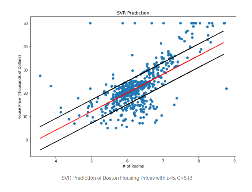
Support Vector Regression

Support Vector Regression lets us define how much error is acceptable in our models in order to find a flexible line of best fit. Rather than minimize error, SVR aims at minimizing the coefficient vectors. The error becomes a constraint rather than an objective function. Some points may fall outside the feasible region, thus necessitating slack variables. The slack variables will represent the deviation from the feasible region, and then will be added to the objective function. This will become hyperparameter C. As C increases, more points are outside the feasible region. Thus, as C increases, MAE tends to decrease. We also need to choose a kernel as a function that maps the data points into a higher dimension. Epsilon will determine the boundary lines of the line of best fit/plane/hyperplane.

Modeling with SVR in Python

from sklearn.model_selection import KFold
kf = KFold(n_splits=10, shuffle=True, random_state=2021)

from sklearn.svm import SVR

svr_rbf = SVR(kernel='rbf', C=100, gamma=0.1, epsilon=.1)
svr_lin = SVR(kernel='linear', C=100, gamma='auto')
svr_poly = SVR(kernel='poly', C=100, gamma='auto', degree=4, epsilon=.1,coef0=1)

model = svr_poly
mae_svr = []

for idxtrain, idxtest in kf.split(dat):
  X_train = dat[idxtrain,0]
  y_train = dat[idxtrain,1]
  X_test  = dat[idxtest,0]
  y_test = dat[idxtest,1]
  model.fit(X_train.reshape(-1,1),y_train)
  yhat_svr = model.predict(X_test.reshape(-1,1))
  mae_svr.append(mean_absolute_error(y_test, yhat_svr))
print("Validated MAE Support Vector Regression = ${:,.2f}".format(1000*np.mean(mae_svr)))

After running the code, the MAE for SVR(poly) is $23,994.88. This means that we may need to modify the parameters or type of model. When we try the linear SVR model, we have an MAE of $4,546.70. This is still a relatively high MAE, but under $5,000. Lastly, if we run the SVR (rbf), we get an MAE of $4,242.04. Thus, the best kernel for this data set is the rbf kernel.

Neural Network

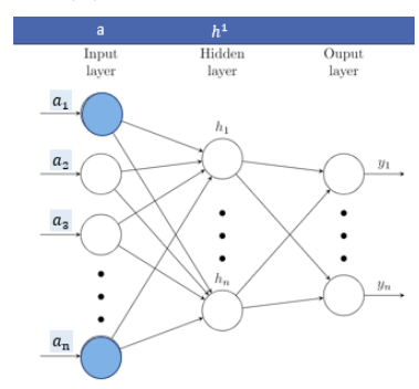
Neural Networks are made up of neurons, or small units which hold a number. These neurons are connected to each other in layers and are assigned an activation value. Each activation number is multiplied with a corresponding weight which describes connection strength from node to node. A neural network has an architecture of input nodes, output nodes, and hidden layers. For each node in a proceeding layer, the weighted sum is computed:

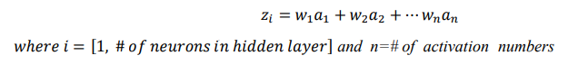
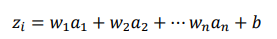
The weighted inputs are added with a bias term in order for the output to be meaningfully active.

The weights and biases of each node are then multiplied against their corresponding activation number. This is repeated throughout the nodes in the hidden layers.

The Activation Function

The function 𝑧𝑖 is linear in nature; thus, a nonlinear activation function is applied for more complex performance. Activation functions commonly used include sigmoid functions, piecewise functions, gaussian functions, tangent functions, threshold functions, or ReLu functions.

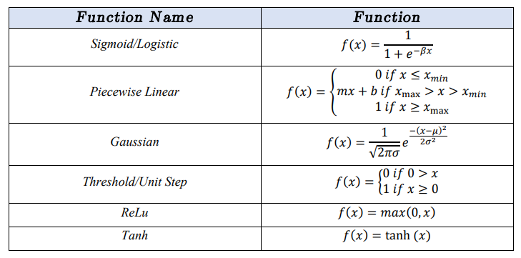
Activation function choice depends on the range needed for the data, error, and speed. Without an activation function, the neural network behaves like a linear regression model.

The Loss Function

A neural network may have thousands of parameters. Some combinations of weights and biases will produce better output for the model. In order to measure error, a loss function is necessary. The loss function tells the machine how far away the combination of weights and biases is from the optimal solution. There are many loss functions that can be used in neural networks; Mean Squared Error and Cross Entropy Loss are two of the most common

Modeling a Neural Network in Python

We must first import all necessary libraries.

import keras
from keras.models import Sequential
from keras.layers import Dense
from keras.layers import Dropout
from sklearn.metrics import r2_score
from keras.optimizers import Adam
from keras.callbacks import EarlyStopping
from sklearn.preprocessing import LabelEncoder 

The variables/features must be designated, and the training and testing data must be split.

X = np.array(df['rooms']).reshape(-1,1)
y = np.array(df['cmedv']).reshape(-1,1)
dat = np.concatenate([X,y.reshape(-1,1)], axis=1)

from sklearn.model_selection import train_test_split as tts
X_train, X_test, y_train, y_test = tts(X, y, test_size=0.3, random_state=2021)

y_train = y_train.reshape(len(y_train),)
y_test = y_test.reshape(len(y_test),)

dat_train = np.concatenate([X_train,y_train.reshape(-1,1)], axis=1)
dat_train = dat_train[np.argsort(dat_train[:, 0])]

dat_test = np.concatenate([X_test,y_test.reshape(-1,1)], axis=1)
dat_test = dat_test[np.argsort(dat_test[:, 0])]

Lastly, the neural network’s architecture must be designed. This particular DNN has four total layers all with the ReLu activation function with exception of the final output layer. The loss function chosen is MSE and the optimizer is Adam.

# Create a Neural Network model
model = Sequential()
model.add(Dense(128, activation="relu", input_dim=1))
model.add(Dense(32, activation="relu"))
model.add(Dense(8, activation="relu"))
# Since the regression is performed, a Dense layer containing a single neuron with a linear activation function.
# Typically ReLu-based activation are used but since it is performed regression, it is needed a linear activation.
model.add(Dense(1, activation="linear"))

# Compile model: The model is initialized with the Adam optimizer and then it is compiled.
model.compile(loss='mean_squared_error', optimizer=Adam(lr=1e-3, decay=1e-3 / 200))

# Patient early stopping
es = EarlyStopping(monitor='val_loss', mode='min', verbose=1, patience=1000)

# Fit the model
history = model.fit(X_train, y_train, validation_split=0.3, epochs=1000, batch_size=100, verbose=0, callbacks=[es])

# Calculate predictions
yhat_nn = model.predict(dat_test[:,0])

In order to measure the accuracy of our model, we will be using MAE once again:

from sklearn.metrics import mean_absolute_error

yhat_nn = model.predict(dat_test[:,0])
mae_nn = mean_absolute_error(dat_test[:,1], yhat_nn)
print("MAE Neural Network = ${:,.2f}".format(1000*mae_nn))

The MAE of this particular neural network is $3,895.49. Although some of the LOWESS models performed better, our DNN may be able to get better if we change the architecture.

Extreme Gradient Boost

Extreme Gradient Boost attempts to help against overfitting by using gradient boosted decision trees. A booster corrects the errors made by an existing model by sequentially adding until no further improvement can be made. Gradient boosting calculates the residuals of each sample and then decides the best split along a given feature. These splits will create trees with the residual values in each leaf. XGBoosting calculates a gain function which keeps track of improvement in accuracy brought about by a split. Thus, we eventually find a threshold that results in the maximum gain. This process is repeated throughout each of the leaves.

Modeling with XGBoost in Python

import xgboost as xgb
model_xgb = xgb.XGBRegressor(objective ='reg:squarederror',n_estimators=100,reg_lambda=20,alpha=1,gamma=10,max_depth=3)

mae_xgb = []

for idxtrain, idxtest in kf.split(dat):
  X_train = dat[idxtrain,0]
  y_train = dat[idxtrain,1]
  X_test  = dat[idxtest,0]
  y_test = dat[idxtest,1]
  model_xgb.fit(X_train.reshape(-1,1),y_train)
  yhat_xgb = model_xgb.predict(X_test.reshape(-1,1))
  mae_xgb.append(mean_absolute_error(y_test, yhat_xgb))
print("Validated MAE XGBoost Regression = ${:,.2f}".format(1000*np.mean(mae_xgb)))

The MAE results as $4,136.63, thus putting it in range with the other models.

Conclusion

MAE’s for each Model

• Linear Regression: $4,109.44
• Epanechnikov Kernel LOWESS : $3,860.55
• Quartic Kernel LOWESS: $3,889.25
• Tri-Cubic Kernel LOWESS: $3,888.18
• SVR Model (linear): $4,546.70
• SVR Model (rbf): $4,242.04
• SVR Model (poly): $23,994.88
• Neural Network: $3,895.49
• XGBOOST: $4,136.63

As can be seen by the data, the LOwESS models had the best accuracy for this data set in terms of mean absolute error. In particular, the Epanechnikov Kernel LOWESS had the best results with an MAE of $3,860.55. The Neural Network’s error was quite close to the other LOWESS models, signifying that if improved, it may be a good candidate for prediction of this data set. The worst model by far was the SVR model with a polynomial kernel. This could possibly be explained by the fact that polynomial kernels tend to overfit many types of data. Although the overall goal of this project was classified as a regression model problem, I would argue that the overfitting could largely be due to the models being univariate and also ignoring the very important factor of time. This problem could perhaps be reshaped as a forecasting problem, as inflation and deflation that occur over time could be creating confusion in the data.